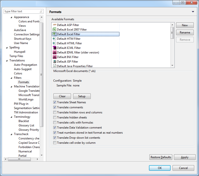
There are two default filters for Excel: Default Excel filter, and Default
Excel 2007 filter. The steps for adding both filters are the same. In
the example below, a Default Excel filter will be added.
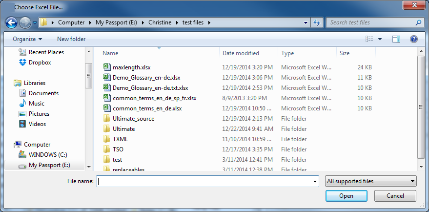
Follow steps 1 to 6 from Adding an Excel file filter.
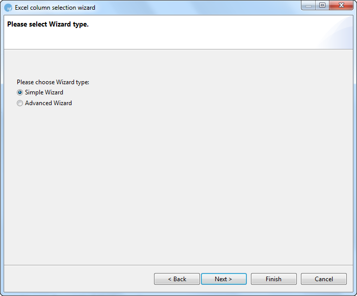
Select Simple Wizard and click
Next.
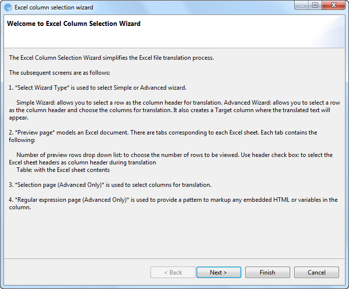
The Preview page appears.
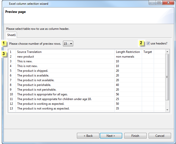
The content in the Preview page is selected for translation.
The Preview page models an Excel file.
Number |
Use |
|

|
Please
choose number of preview rows drop down list: |
select
the number of rows to show on the preview page. |

|
Use
headers check box: |
use
the column headers of the Excel sheet. If not selected, the
column letter (A,B, C) appears in the next step. |

|
Table
with the Excel sheet contents |
select
the first row for translation. Rows above the selected row
will not be translated. |
Click Finish.
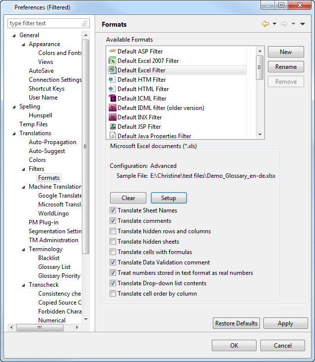
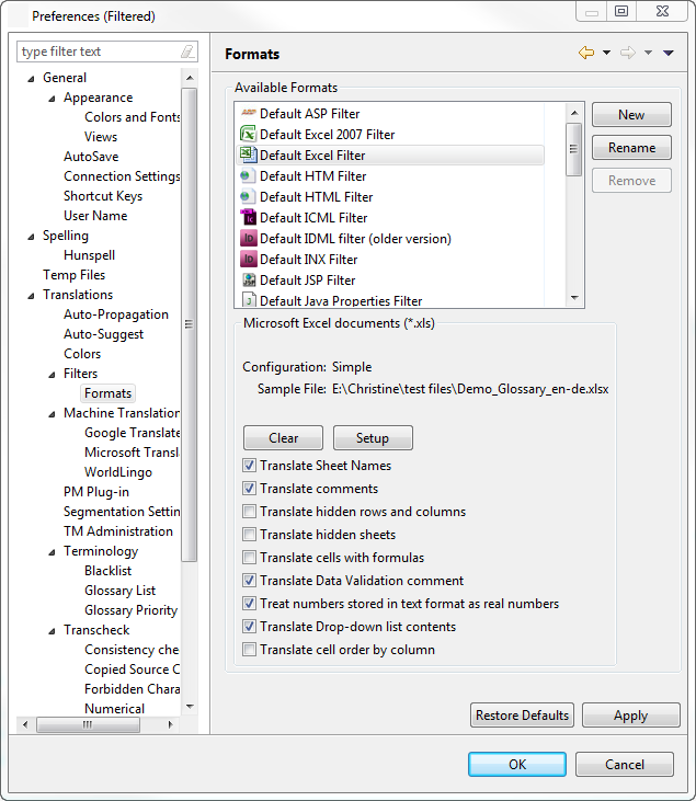
The configuration and sample file path appears in the Formats options
box as shown in the screenshot below.
Select the Translate
Sheet Names checkbox to include sheet names as translatable
text. Selected by default.
Select Translate
Comments to clear it, and not include comments as translatable
text. Selected by default.
Select the Translate
hidden rows and columns checkbox to include rows and columns
hidden in the Excel file as translatable text.
Select Translate
hidden sheets to include hidden Excel sheets.
Select the Translate
cell with formulas checkbox to include cells with notes and
formulas as translatable text.
Select Translate
Data Validation comment to clear it, and not include columns
in the Excel sheet used to record comments validating the data, for
example, columns recording vaccination data by date applied and dosage.
Selected by default.
Select the Treat
numbers stored in text format as real numbers checkbox to include
numbers as translatable text. Selected by default.
Select Translate
Drop-down list contents to include the drop-down list contents
in the translation. Selected by default.
Select Translate
cell order by column to extract cells by columns, instead of
by rows.
Follow steps 1 to 6 from Adding an Excel file filter.
The Preview page appears.
The content in the Preview page is selected for translation.
The Preview page models an Excel file.
Number |
Use |
|
|
Please
choose number of preview rows drop down list: |
select
the number of rows to show on the preview page. |
|
Use
headers check box: |
use
the column headers of the Excel sheet. If not selected, the
column letter (A,B, C) appears in the next step. |
|
Table
with the Excel sheet contents |
select
the first row for translation. Rows above the selected row
will not be translated. |
Click Next
The Selection page appears. If you have selected the Use
header checkbox, the Excel sheet headers appear as column names,
in the Column Name column.
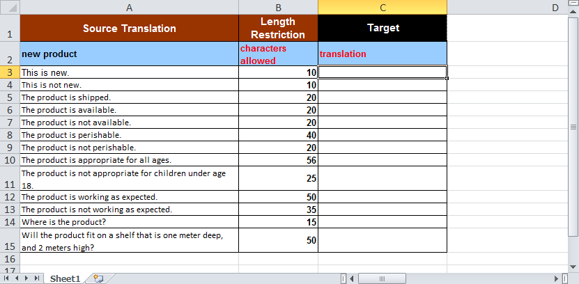
In the example below, the Excel sheet headers are Source Translation,
Length Restriction, and Target. An example of the source Excel spreadsheet
appears below.
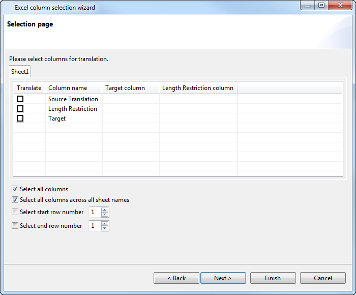
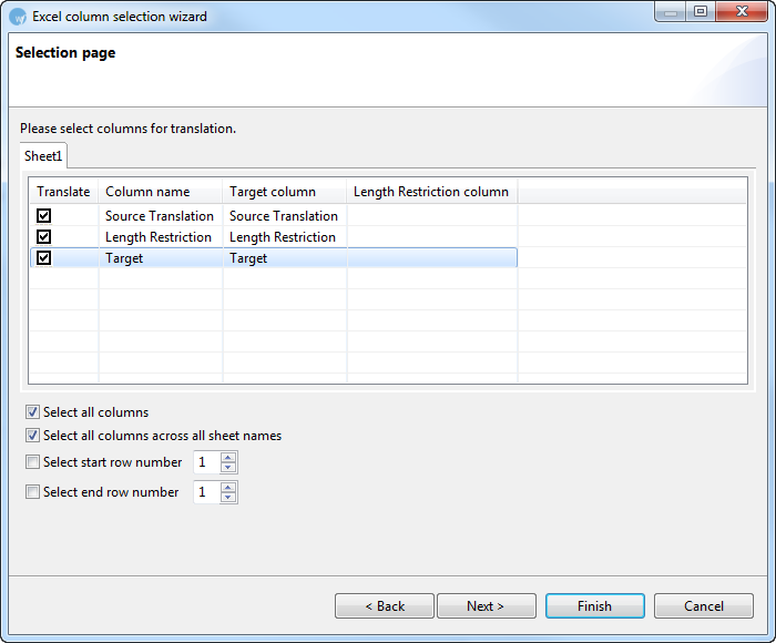
In the Translate
column on the Selection page, select the columns for translation.
Select the starting row number.
The content extract begins with this row number, and ends at the selected
end row number.
Select the end row number. The content
extract ends with this row number, having begun at the selected end
row number.
The corresponding Column name appears in the Target column as shown
in the example.
Select the Translate
Sheet Names checkbox to include sheet names as translatable
text. Selected by default.
Select Translate
Comments to include comments as translatable text. Selected
by default.
Select the Translate
hidden rows and columns checkbox to include rows and columns
hidden in the Excel file as translatable text.
Select Translate
hidden sheets to include hidden Excel sheets.
Select the Translate
cell with formulas checkbox to include cells with notes and
formulas as translatable text.
Select Translate
Data Validation comment to clear it, and not include columns
in the Excel sheet used to record comments validating the data, for
example, columns recording vaccination data by date applied and dosage.
Selected by default.
Select the Treat
numbers stored in text format as real numbers checkbox to clear
it, and not include numbers as translatable text. Selected by default.
Select Translate
Drop-down list contents to include the drop-down list contents
in the translation. Selected by default.
Select Translate
cell order by column to extract cells by columns, instead
of by rows.